Line

Used to track changes over time and also compare with other changes (more lines within the same plot). Better than bar charts for small changes.

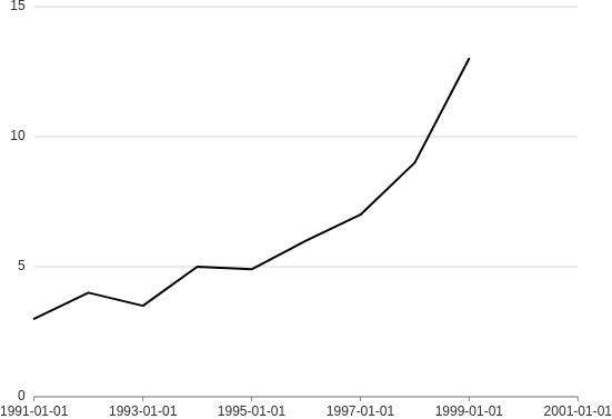
from h2o_wave import data

q.page['example'] = ui.plot_card(
    box='1 1 4 5',
    title='Line',
    data=data('year value', 8, rows=[
        ('1991', 3),
        ('1992', 4),
        ('1993', 3.5),
        ('1994', 5),
        ('1995', 4.9),
        ('1996', 6),
        ('1997', 7),
        ('1998', 9),
        ('1999', 13),
    ]),
    plot=ui.plot([ui.mark(type='line', x_scale='time', x='=year', y='=value', y_min=0)])
)

Check the full API at ui.plot_card.

Groups

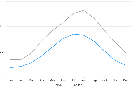
Use the color attribute to group by a categorical column.

from h2o_wave import data

q.page['example'] = ui.plot_card(
    box='1 1 4 5',
    title='Line, groups',
    data=data('month city temperature', 24, rows=[
        ('Jan', 'Tokyo', 7),
        ('Jan', 'London', 3.9),
        ('Feb', 'Tokyo', 6.9),
        ('Feb', 'London', 4.2),
        ('Mar', 'Tokyo', 9.5),
        ('Mar', 'London', 5.7),
        ('Apr', 'Tokyo', 14.5),
        ('Apr', 'London', 8.5),
        ('May', 'Tokyo', 18.4),
        ('May', 'London', 11.9),
        ('Jun', 'Tokyo', 21.5),
        ('Jun', 'London', 15.2),
        ('Jul', 'Tokyo', 25.2),
        ('Jul', 'London', 17),
        ('Aug', 'Tokyo', 26.5),
        ('Aug', 'London', 16.6),
        ('Sep', 'Tokyo', 23.3),
        ('Sep', 'London', 14.2),
        ('Oct', 'Tokyo', 18.3),
        ('Oct', 'London', 10.3),
        ('Nov', 'Tokyo', 13.9),
        ('Nov', 'London', 6.6),
        ('Dec', 'Tokyo', 9.6),
        ('Dec', 'London', 4.8),
    ]),
    plot=ui.plot([ui.mark(type='line', x='=month', y='=temperature', color='=city', y_min=0)])
)

Curves

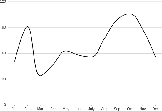
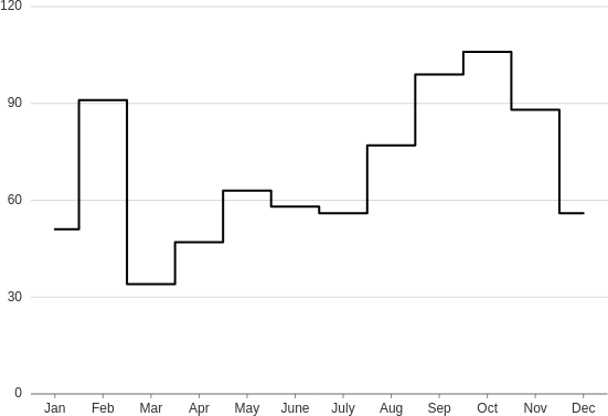
Don't like sharp edges? Just play around with curve attribute. Allowed values are smooth, step, step-after and step-before.

Smooth

from h2o_wave import data

q.page['example'] = ui.plot_card(
    box='1 1 4 5',
    title='Line, smooth',
    data=data('month price', 12, rows=[
        ('Jan', 51),
        ('Feb', 91),
        ('Mar', 34),
        ('Apr', 47),
        ('May', 63),
        ('June', 58),
        ('July', 56),
        ('Aug', 77),
        ('Sep', 99),
        ('Oct', 106),
        ('Nov', 88),
        ('Dec', 56),
    ]),
    plot=ui.plot([
        ui.mark(type='line', x='=month', y='=price', curve='smooth', y_min=0)
    ])
)

Step

from h2o_wave import data

q.page['example'] = ui.plot_card(
    box='1 1 4 5',
    title='Line, step',
    data=data('month price', 12, rows=[
        ('Jan', 51),
        ('Feb', 91),
        ('Mar', 34),
        ('Apr', 47),
        ('May', 63),
        ('June', 58),
        ('July', 56),
        ('Aug', 77),
        ('Sep', 99),
        ('Oct', 106),
        ('Nov', 88),
        ('Dec', 56),
    ]),
    plot=ui.plot([
        ui.mark(type='line', x='=month', y='=price', curve='step', y_min=0)
    ])
)

Step after

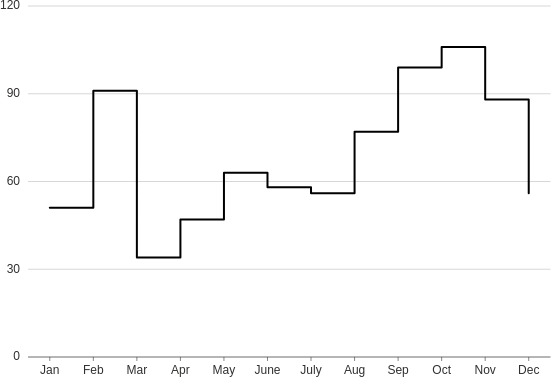
from h2o_wave import data

q.page['example'] = ui.plot_card(
    box='1 1 4 5',
    title='Line, step-after',
    data=data('month price', 12, rows=[
        ('Jan', 51),
        ('Feb', 91),
        ('Mar', 34),
        ('Apr', 47),
        ('May', 63),
        ('June', 58),
        ('July', 56),
        ('Aug', 77),
        ('Sep', 99),
        ('Oct', 106),
        ('Nov', 88),
        ('Dec', 56),
    ]),
    plot=ui.plot([
        ui.mark(type='line', x='=month', y='=price', curve='step-after', y_min=0)
    ])
)

Step before

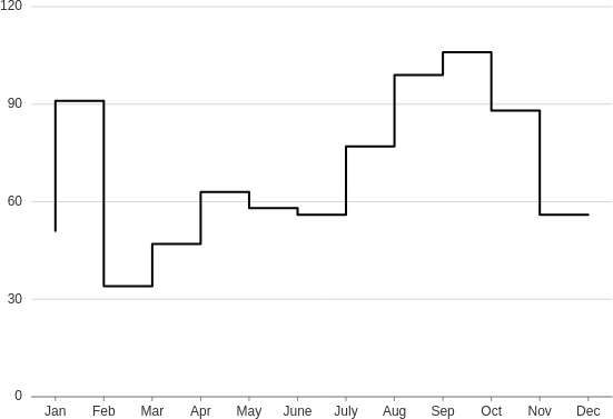
from h2o_wave import data

q.page['example'] = ui.plot_card(
    box='1 1 4 5',
    title='Line, step before',
    data=data('month price', 12, rows=[
        ('Jan', 51),
        ('Feb', 91),
        ('Mar', 34),
        ('Apr', 47),
        ('May', 63),
        ('June', 58),
        ('July', 56),
        ('Aug', 77),
        ('Sep', 99),
        ('Oct', 106),
        ('Nov', 88),
        ('Dec', 56),
    ]),
    plot=ui.plot([
        ui.mark(type='line', x='=month', y='=price', curve='step-before', y_min=0)
    ])
)

Labels

Add labels to a line plot.

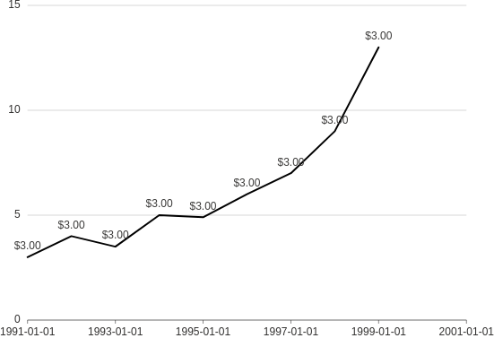
from h2o_wave import data

q.page['example'] = ui.plot_card(
    box='1 1 4 5',
    title='Line, labels',
    data=data('year price', 9, rows=[
        ('1991', 3),
        ('1992', 4),
        ('1993', 3.5),
        ('1994', 5),
        ('1995', 4.9),
        ('1996', 6),
        ('1997', 7),
        ('1998', 9),
        ('1999', 13),
    ]),
    plot=ui.plot([
        ui.mark(type='line', x_scale='time', x='=year', y='=price', y_min=0,
                label='=${{intl price minimum_fraction_digits=2 maximum_fraction_digits=2}}')
    ])
)

Custom labels

Customize label rendering as you see fit.

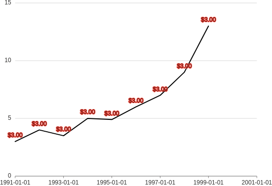
from h2o_wave import data

q.page['example'] = ui.plot_card(
    box='1 1 4 5',
    title='Line, labels, custom',
    data=data('year price', 9, rows=[
        ('1991', 3),
        ('1992', 4),
        ('1993', 3.5),
        ('1994', 5),
        ('1995', 4.9),
        ('1996', 6),
        ('1997', 7),
        ('1998', 9),
        ('1999', 13),
    ]),
    plot=ui.plot([
      ui.mark(type='line', x_scale='time', x='=year', y='=price', y_min=0,
              label='=${{intl price minimum_fraction_digits=2 maximum_fraction_digits=2}}',
              label_fill_color='rgba(0,0,0,0.65)', label_stroke_color='$red', label_stroke_size=2)
    ])
)